Probability Distributions for Measurement Uncertainty

 
 

Introduction

Probability distributions are an important part of measurement uncertainty analysis that people continually struggle with. Today, my goal is to help you learn more about probability distributions without having to grab a statistics textbook. Although there are hundreds of probability distributions that you could use, I am going to focus on the 6 that you need to know.

If you constantly struggle with probability distributions, keep reading. I am going to explain what are probability distributions, why they are important, and how they can help you when estimating measurement uncertainty.

In this guide, I am going to cover the following information. You can jump ahead by clicking the links below

 

 
 

What is a Probability Distribution

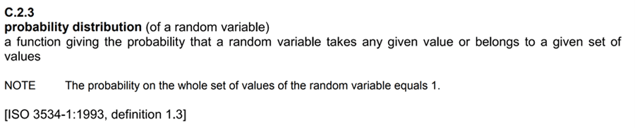
According to JCGM 100:2008 Definition C.2.3, a probability distribution is a function giving the probability (likelihood) that a random variable takes any given value or belongs to a given set of values.

Look at the below image to see the definition from the GUM.

 
Simply explained, probability distributions are a function, table, or equation that shows the relationship between the outcome of an event and its frequency of occurrence.

Probability distributions are helpful because they can be used as a graphical representation of your measurement functions and how they behave. When you know how your measurement function has performed in the past, you can more confidently predict future outcomes.

Before jumping head-first into the different types of probability distribution, let’s first learn a little more about probability distributions. In the next few paragraphs, I am going to explain some characteristics that you should know.

 
 

Histogram

A histogram is a graphical representation used to understand how numerical data is distributed.

Take a look at below image. It is a histogram of a Gaussian or Normal distribution.

 
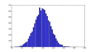
Look at the histogram and see how the majority of the data collected is grouped at the center. This is called central tendency.

Now look at height of each bar in the histogram. The height of the bars indicate how frequent the outcome it represents occurs. The taller the bar, the more frequent the occurrence.

 
 

Skewness

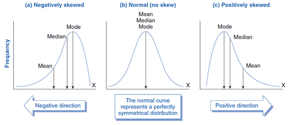
Skewness is a measure of the probability distributions symmetry. Look at the below image to see how probability distributions can skew to the left or the right.

 
 

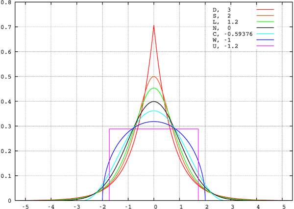
Kurtosis

Kurtosis is a measure of the tailedness and peakedness relative to a normal distribution. As you can see from the image below, distributions with wider tails have smaller peaks while distributions with greater peaks have narrower tails. Do you see the relationship?

 
 

Why is it important

I know it seems like I am making you read more information that you want to know, but it is important to know these details so you can select the appropriate probability distribution that characterizes your data.

If you are uncertain how your data is distributed, create a histogram of your data and compare it to the following probability distributions.

 
 

---

 
 

Probability Distributions for Measurement Uncertainty

Now that you know what is a probability distribution, let’s learn more about different types of distributions. The most commonly used probability distributions for estimating measurement uncertainty are;

• Normal,
• Rectangular,
• Triangle,
• U-Shaped,
• Log-Normal, and
• Rayleigh

In the sections below, you will learn more about each one of these distributions. I will cover general information that you need for estimating measurement uncertainty.

After reading this article, you should be able identify which probability distributions you should use in your uncertainty budget and how to convert your uncertainty contributors to standard deviation equivalents (a critical step to estimating uncertainty).

 
 

Gaussian (a.k.a. Normal) Distribution

 
 

Description

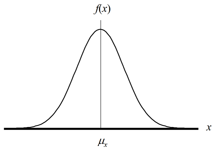
The Normal distribution is a function that represents the distribution of many random variables as a symmetrical bell-shaped graph where the peak is centered about the mean and is symmetrically distributed in accordance with the standard deviation.

This means that outcomes are more likely to occur near the mean or average and spread about the mean where the results further from the mean are less likely to occur.

The normal distribution is the most commonly used probability distribution for evaluating Type A uncertainty data. If you do not know what Type A uncertainty is, it is the data that you collect from experimental testing, such as repeatability, reproducibility, and stability testing.

To get a better understanding, imagine you are going to collect 100 measurement samples and create a histogram graph with your results. The histogram for your data should resemble a shape close to a normal distribution.

According to the Central Limit Theorem, the more data that you collect, the closer your histogram will begin to resemble a normal distribution.

Now, I do not expect you to collect 100 samples every time you perform repeatability and reproducibility test. Instead, I recommend that you begin by collecting 20 to 30 samples for each repeatability test. This should give you a good baseline to begin with and allow you to characterize your data with a normal distribution.

 
 

Divisor for Normal Distribution

To convert a normally distributed uncertainty to a standard deviation equivalent, use the equation given below. Divide the estimated uncertainty (U_i) by its coverage factor (k).

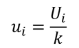
Where,
u_i = standard uncertainty
U_i = expanded uncertainty
k = coverage factor

The value of the coverage factor depends on the level of confidence associated with the uncertainty estimate. In Appendix G of the JCGM 100:2008, Table G.1 will help you find the coverage factor associated with a specific level of confidence.

Look at the image below to see Table G.1 from the GUM.

 
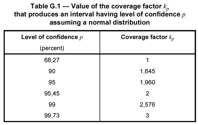
From the table, you can see a standard deviation from a repeatability test would have a 68.27% confidence level and a coverage factor of k=1.

Additionally, you will find that the uncertainty in your calibration reports has a 95.45% confidence level and a coverage factor of k=2.

 
 

Standard Uncertainty Example for Normal Distribution

Example 1: Standard Deviation from Repeatability Test

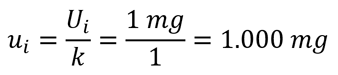
For example, if you collect 20 samples for a repeatability test and calculate the standard deviation, the coverage factor (k) is 1. It is equal to 1 because your standard deviation is expressed at the 1-sigma level of confidence (i.e. 68.27% C.I.).

So, if your standard deviation is 1 mg, then you would divide it by a coverage factor of 1 and your standard uncertainty would be equal to 1 mg.

The result would have no reduction in value because it is already equal to a standard deviation.

Look at the image below to see an example of the calculation.

 
If you calculate measurement uncertainty using Microsoft Excel, then you would use the following formula:

 

 
 

Example 2: Expanded Uncertainty from a Calibration Report

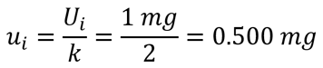
For the next example, imagine you are evaluating the measurement uncertainty from your calibration report. The reported uncertainty should be expressed at a 95% confidence interval where k equals 2 .

If the calibration uncertainty reported in your certificate is 1 mg, then you would divide it by the coverage factor of 2. The resulting standard uncertainty would be equal 0.5 mg.

Look at the image below to see an example of the calculation.

 
If you calculate measurement uncertainty using Microsoft Excel, then you would use the following formula:

 

 
 
 

Rectangular (a.k.a. Uniform) Distribution

 
 

Description

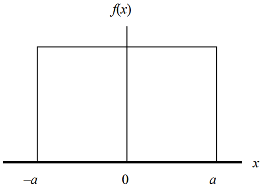
The Rectangular Distribution is a function that represents a continuous uniform distribution and constant probability. In a rectangular distribution, all outcomes are equally likely to occur.

The rectangular distribution is the most commonly used probability distribution in uncertainty analysis. If you are wondering why, it is because it covers the majority of uncertainty factors where the evaluator says, “I am not sure how the data is distributed.”

When you are not confident about how your data is distributed, it is best to evaluate it conservatively.

In this situation, the rectangular distribution is a great default option which is why most ISO/IEC 17025 assessors recommend it. So, make sure to remember the rectangular distribution, you will be using this probability distribution a lot.

 
 

Divisor for Rectangular Distribution

To convert an uncertainty with a rectangular distribution to a standard deviation equivalent, use the equation given below. Divide the estimated uncertainty (U_i) by the square root of three (3).

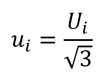
Where,
u_i = standard uncertainty
U_i = expanded uncertainty

 
Alternatively, you can encounter a rectangular distribution where you believe the value (x_i) is the midpoint of the distribution (or half the distribution). When this happens, divide the estimated uncertainty (U_i) by two times the square root of three (3).

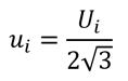
Where,
u_i = standard uncertainty
U_i = expanded uncertainty

 
Otherwise, you could divide the uncertainty (U_i) by the square root of twelve (12). Mathematically, the result is the same.

 
 

Standard Uncertainty Example for Rectangular Distribution

Example 1: Resolution of a Measurement Equipment

For example, if you a digital multimeter with a resolution of 1 mV, then you would characterize the instrument resolution with a rectangular distribution and convert the uncertainty (U_i) to a standard uncertainty (u_i) by dividing the uncertainty by the square root of three.

 
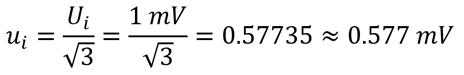
If you calculate measurement uncertainty using Microsoft Excel, then you would use the following formula:

 

 
 

Example 2: Half-Resolution of a Measurement Equipment

Now, imagine you a digital multimeter with a resolution of 1 mV and you want to consider the uncertainty (U_i) as half of the resolution (0.5R).

Then, characterize the instrument resolution with a rectangular distribution and convert the uncertainty (U_i) to a standard uncertainty (u_i) by dividing the uncertainty by the square root of twelve.

 
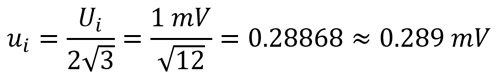
If you calculate measurement uncertainty using Microsoft Excel, then you would use the following formula:

 

 
 
 

Triangle Distribution

 
 

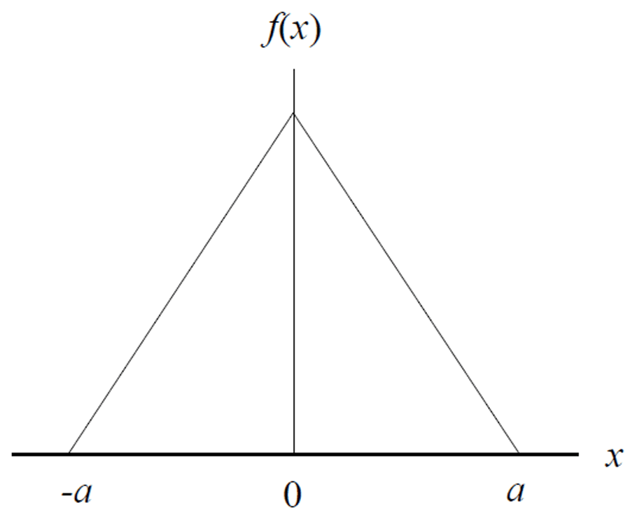
Description

The Triangle Distribution is a function that represents a known minimum, maximum, and estimated central value.

Similar to the rectangular distribution, the triangle distribution is referred to as a “lack of knowledge” distribution. You may not know where the value (x_i) is within the interval, but you think it is closer to the mean (or center of the interval) than the limits.

According to the JCGM 100:2008, it is recommended as an alternative to the rectangular distribution because it is a more realistic expectation.

I will cover more about this later in the next section on GUM recommendations.

 
 

Divisor for Triangle Distribution

To convert an uncertainty with a Triangle distribution to a standard deviation equivalent, use the equation given below. Divide the estimated uncertainty (U_i) by the square root of six (6).

Where,
u_i = standard uncertainty
U_i = expanded uncertainty

 
 

Standard Uncertainty Example for Triangle Distribution

Example 1: Manufacturer Specification

For example, if you are using a calibrated mass with a maximum permissible error (MPE) of 1 mg, then you could characterize the uncertainty with a triangle distribution and convert the uncertainty (U_i) to a standard uncertainty (u_i) by dividing the uncertainty by the square root of six.

 
If you calculate measurement uncertainty using Microsoft Excel, then you would use the following formula:

 

 
 
 

U-shaped Distribution

 
 

Description

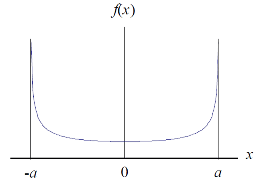
The U-shaped Distribution is a function that represents outcomes that are most likely to occur at the extremes of the range. The distribution forms the shape of the letter ‘U,’ but does not necessarily have to be symmetrical.

The U-shaped distribution is helpful where events frequently occur at the extremes of the range.

Consider the thermostat that controls the temperature of your laboratory. Typically, most thermostat controllers only attempt to control temperature by start and stopping your HVAC system at the extremes of the range.

 
 

Temperature Example for U-Shaped Distribution

For example, imagine that your laboratory thermostat is set at 20°C and controls the temperature to ±1°C. Most likely, your thermostat does not activate your HVAC system until the laboratory temperature reaches either 19°C or 21°C. This means that your laboratory is not normally at 20°C. Instead, your laboratory temperatures are dwelling around the limits of the thermostat’s thresholds before activating or deactivating.

For this reason, you could characterize your laboratory temperature data using a U-shaped distribution. However, most people prefer to use a rectangular or triangle distribution for uncertainties related to environmental temperature.

 
 

RF Power Example for U-Shaped Distribution

Another common example of using a U-shaped distribution is mismatch uncertainty in RF/Microwave measurement functions.

Look at the image below to see the table of recommended probability distributions from Keysight’s Guide: “Fundamentals of RF and Microwave Power Measurements (Part 3).”

 
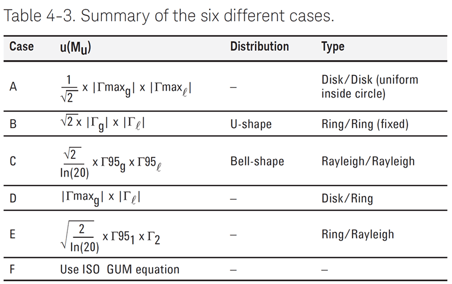
The above table also includes recommendations for the Rayleigh Distribution. I will discuss this more in the next section.

 
 

Divisor for U-Shaped Distribution

To convert an uncertainty with a U-Shaped distribution to a standard deviation equivalent, use the equation given below. Divide the estimated uncertainty (Ui) by the square root of two (2).

Where,
u_i = standard uncertainty
U_i = expanded uncertainty

 
 

Standard Uncertainty Example for U-Shaped Distribution

Example 1: Mismatch Uncertainty

Imagine you are using an RF Power sensor to measure the output power level of a signal generator. If the mismatch uncertainty between the sensor and the source is estimated to be 1 µW, then characterize the uncertainty with a U-shaped distribution and convert the uncertainty (U_i) to a standard uncertainty (u_i) by dividing the uncertainty by the square root of two.

 
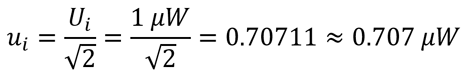
If you calculate measurement uncertainty using Microsoft Excel, then you would use the following formula:

 

 
 
 

Rayleigh Distribution

 
 

Description

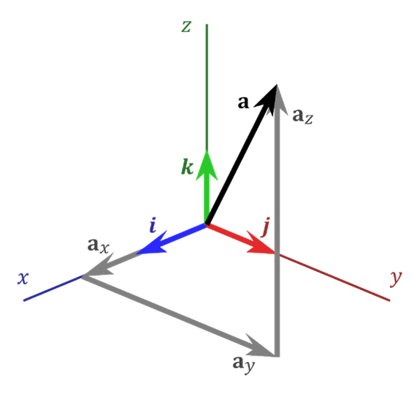
Rayleigh distributions are used when the magnitude of a vector is associated with it’s directional components (e.g. x and y), which can include both real and imaginary components (e.g. i and j).

When the directional components are orthogonal (i.e. statistically independent) and normally distributed, the resulting vector will have a Rayleigh distribution.

 
 

Common Uses of the Rayleigh Distribution

Rayleigh distributions are commonly used in electrical metrology for RF and Microwave functions. Additionally, they are commonly used in other areas of metrology where two vectors are involved.

For example, when wind velocity is analyzed by its two dimensional vector components, x and y, the resulting vector has a Rayleigh distribution. For this to happen, x and y must be orthogonal and normally distributed.

Another example of using a Rayleigh distribution to characterize mismatch uncertainty.

In the previous section, I showed you that you can characterize mismatch uncertainty with a U-Shaped distribution. However, Keysight’s Guide: “Fundamentals of RF and Microwave Power Measurements (Part 3)” states the U-shaped distribution is likely to overstate your uncertainty. So, they recommend the using the Rayleigh distribution to characterize mismatch uncertainty because it is more realistic.

Look at the image below to see the recommendation for using the Rayleigh distribution from Keysight’s Guide: “Fundamentals of RF and Microwave Power Measurements (Part 3).”

 
 

Divisor for Rayleigh Distribution

To convert an uncertainty with a Rayleigh distribution to a standard deviation equivalent, use the equation given below. Divide the estimated uncertainty (Ui) by the square root of two times the natural logarithm of 20.

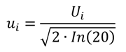
Where,
u_i = standard uncertainty
U_i = expanded uncertainty
ln = natural logarithim

In many cases, you will need to know the measurement uncertainty of each directional component to calculate the measurement uncertainty of the vector component. Afterward, you can use the above equation to reduce your uncertainty component to a standard deviation equivalent.

For a better explanation, click the link below to read this paper by Michael Dobbert from Keysight Technologies.

• Revisiting Mismatch Uncertainty with the Rayleigh Distribution

 
 

Standard Uncertainty Example for Rayleigh Distribution

Example 1: Mismatch Uncertainty

Imagine you are using an RF Power sensor to measure the output power level of a signal generator. If the mismatch uncertainty between the sensor and the source is estimated to be 1 µW, then characterize the uncertainty with a Rayleigh distribution and convert the uncertainty (U_i) to a standard uncertainty (u_i) by dividing the uncertainty by the square root of two times the natural logarithm of 20.

 
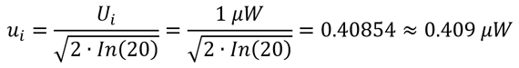
If you calculate measurement uncertainty using Microsoft Excel, then you would use the following formula:

 

 
 
 

Log-Normal Distribution

 
 

Description

The log-normal distribution is a function of a natural logarithm that is normally distributed.

The log-normal distribution is a probability distribution that is commonly encountered but rarely used. Most of the time, it is not used due of lack of knowledge or lack of software needed to properly evaluate the data. Therefore, most people use the Normal Distribution instead.

However, Log-Normal distributions are great for characterizing:

• Asymmetric tolerance limits,
• Measurements constrained by physical limits (e.g. gauge block),
• Microbiology plate counts (CFU), and
• Curve-fitting coefficients.

 
 

Common Uses of the Log-Normal Distribution

For example, many length, height, weight, and concentration measurements can have physical limitations. Therefore, you are likely to end up with measurement results and uncertainties that should be characterized with a log-normal distribution.

Imagine you are measuring the length of a gauge block. After performing repeated measurements, you are likely to see more results that are larger than the actual length of the gauge block than the number of results smaller than it. This is due to the length of the gauge block being constrained to it’s physical limits.

Similar results are likely to occur if you measure the weight of a calibrated mass. You are likely to record more results greater than the actual mass and fewer results less than the actual mass. Again, this is due to the mass being constrained to it’s physical limits.

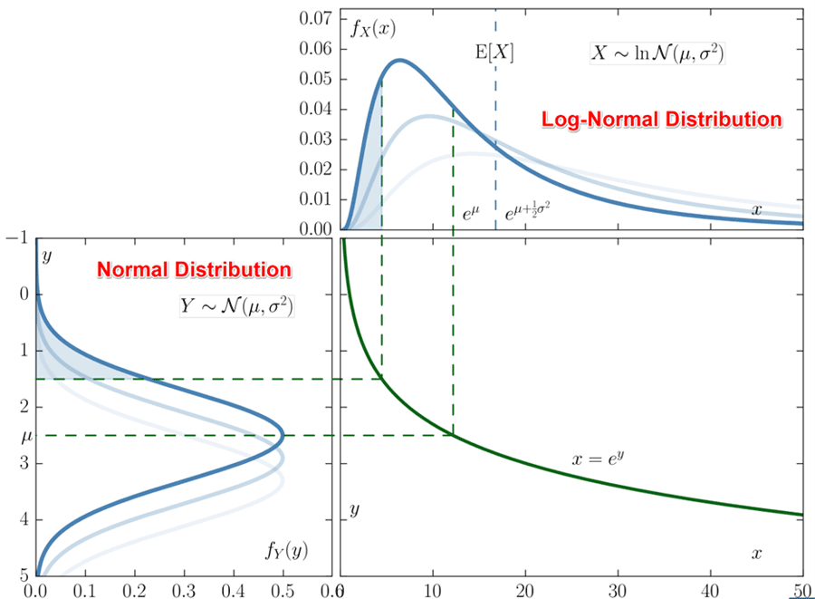
In other situations, you may have measurement results that are normally distributed but are related to a log-normal function.

Look at the image below to see the relationship between normal and log-normal distributions.

 
 

Divisor for Log-Normal Distribution

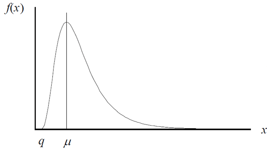
To convert an uncertainty with a Log-Normal distribution to a standard deviation equivalent, use the equation given below. Most likely, you will need software to help you calculate this. Additionally, you will need to know the median, shape parameter, and the physical limit

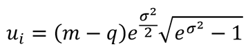
Where,
u_i = standard uncertainty
m = median (scale parameter)
q = physical limit
σ = shape parameter

 
You can learn more about the Log-Normal distribution from the following sources:

• NIST SEMATECH, Section 1.3.6.6.9, “Lognormal Distribution”
• Integrated Sciences Group, “Error Distribution Variances and Other Statistics”

 
Alternatively, I found a paper from Fluke Calibration that used a Log-Normal distribution in an uncertainty budget. The divisor Fluke used to convert uncertainty to a standard deviation equivalent was 2.375.

Now, I recommend this method as an easier option. Look at the equation below.

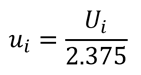
Where,
u_i = standard uncertainty
U_i = expanded uncertainty

 
 

Standard Uncertainty Example for Log-Normal Distribution

Example 1: Measuring a Gauge Block with a Caliper

Imagine you are using a caliper to measure the length of a gauge block and the uncertainty is 1 µm with a Log-Normal distribution. Convert the uncertainty to a standard deviation by dividing it by 2.375.

 
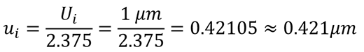
If you calculate measurement uncertainty using Microsoft Excel, then you would use the following formula:

 

 
 

---

 
 

How to Pick Probability Distributions –
Recommendations from the GUM with Decision Rules

In this section, I am going to show you and explain the recommendations from the JCGM 100:2008 (i.e. GUM) so you can pick the right probability distribution. The GUM recommends the following distributions and provides guidance on recommend use cases.

1. Normal Distribution,
2. Rectangular Distribution,
3. Trapezoid Distortion, and
4. Triangle Distribution

 
 

Normal Distribution

According to the JCGM 100:2008, there are 3 conditions which it is recommended to select a Normal Distribution. These are 4 conditions include:

1. Standard Deviation,
2. Multiple of a Standard Deviation,
3. Level of Confidence, or
4. Combination of Multiple Factors

 
 

A) Standard Deviation

If your uncertainty is a standard deviation or standard deviation of the mean, then select a Normal distribution.

 

 
 
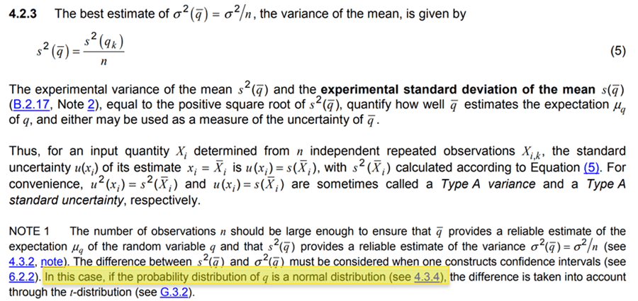
According to the JCGM 100:2008, sections 4.2.3 and G2.2 discuss the probability distribution of a mean and variance (or standard deviation) is a normal distribution.

Look at the image below to see an excerpt from JCGM 100:2008, section 4.2.3.

 
Look at the image below to see an excerpt from JCGM 100:2008, section G.2.2.

 
 

B) Multiple of a Standard Deviation

If your uncertainty is expressed as a multiple of a standard deviation, then select a Normal distribution.

 

 
 
According to the JCGM 100:2008, section 4.3.3 states if an estimate of uncertainty is stated to be a particular multiple of a standard deviation, the standard uncertainty is simply the quoted value divided by the multiplier, and the estimated variance is the square of the quotient.

From the GUM statement, the standard uncertainty is considered a standard deviation (i.e. square-root of the variance). Therefore, it is recommended to select a normal distribution.

Look at the image below to see an excerpt from JCGM 100:2008, section 4.3.3.

 
 

C) Uncertainty Expressed at a Confidence Interval

If your uncertainty is expressed at a specific level of confidence, then select a Normal distribution.

 

 
 
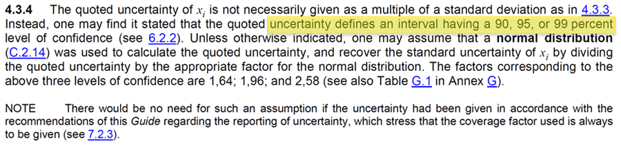
According to the JCGM 100:2008, section 4.3.4 states “the quoted uncertainty of x_i is not necessarily given as a multiple of a standard deviation. Instead, one may find it stated that the quoted uncertainty defines an interval having a 90, 95, or 99 percent level of confidence. Unless otherwise indicated, one may assume that a normal distribution was used to calculate the quoted uncertainty…”

From the GUM statement, an uncertainty expressed at particular level of confidence can be assumed to have a normal distribution.

Look at the image below to see an excerpt from JCGM 100:2008, section 4.3.4.

 
 

D) Uncertainty Expressed at a Combination of Factors

If your uncertainty is expressed as a combination of several contributing factors, then select a Normal distribution.

 

 
 
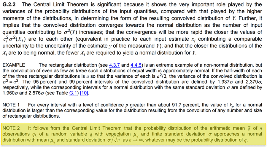
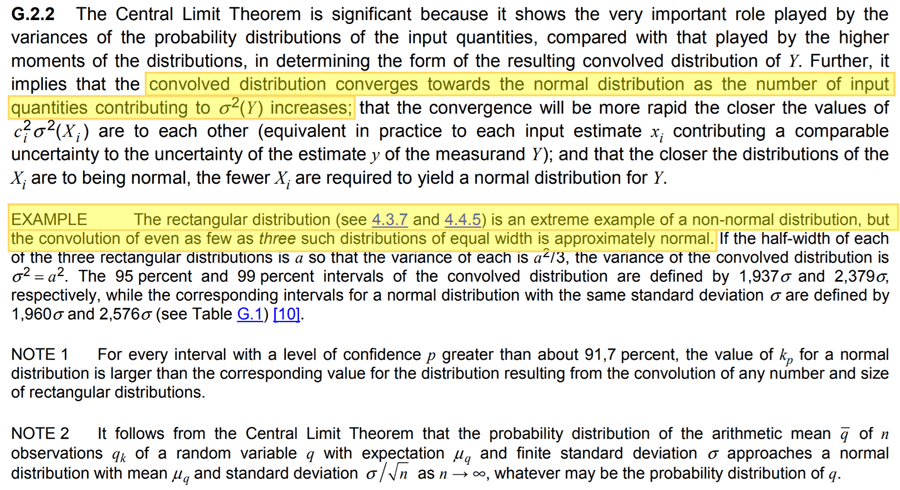
This is recommended in Appendix G of the JCGM 100:2008. In section G.2.2, the GUM provides information on the Central Limit Theorem.

When several sources of uncertainty, each with there own probability distribution, are combined, the resulting distribution is a Normal distribution.

The example at the bottom of the section describes combining as few as three rectangular distributions will still result in a Normal distribution.

Look at the image below to see section G.2.2 from the JCGM 100:2008.

 
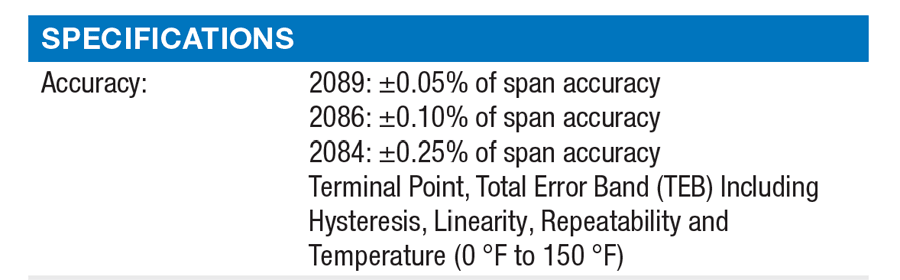
In the image below, you will see a datasheet for a digital pressure gauge that states the accuracy specification is based on the combination of several factors. Even though the datasheet does not state a confidence level or multiple of a standard deviation, you can still assume a Normal distribution based on the Central Limit Theorem.

 
 

Rectangular Distribution

Summary: Limits with No Knowledge of Possible Values or Limits with Expected Value Near Limits

If your uncertainty is estimated only by limits and there is no specific knowledge about the possible values within the interval, then one can assume a rectangular distribution.

 

 
 
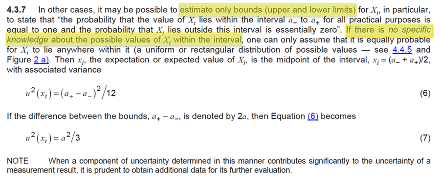
According to the JCGM 100:2008, section 4.3.7 states “In other cases, it may be possible to estimate only bounds (upper and lower limits) for X_i, in particular, to state that “the probability that the value of X_i lies within the interval a- to a+ for all practical purposes is equal to one and the probability that X_i lies outside the interval is essentially zero.” If there is no specific knowledge about the possible values of X_i within the interval, one can only assume that it is equally probable for X_i to lie anywhere within it (a uniform or rectangular distribution of possible values).”

From the GUM statement, an uncertainty expressed only by limits with no knowledge of the actual value within the limits can be assumed to have a rectangular distribution.

This is applicable to tolerance limits, acceptance limits, maximum permissible error, etc.

Now, many guides, professionals, and assessors claim that manufacturers specifications and tolerances should be characterized by a rectangular distribution unless it meets the criteria for normal distributions above. If you follow what is written in the GUM, the rectangular distribution only applies if you estimate the uncertainty on only limits with no consideration or knowledge about the calibrated or certificate value.

However, if your equipment is calibrated and you know where the calibrated or certificate value lies within the limits, then you may be able to use a different distribution. Make sure to read the next section to learn more.

Look at the image below to see an excerpt from JCGM 100:2008, section 4.3.7.

 
 

Triangle and Trapezoid Distribution

Summary: Alternative to the Rectangular Distribution

Since a rectangular distribution is an extreme and unrealistic distribution, the GUM proposes alterative options in section 4.3.9.

If your uncertainty is estimated only by limits and there is no specific knowledge about the possible values within the interval but you expect values are more likely to be closer to the midpoint than the limits, then you can assume a trapezoid or a triangle distribution.

 

 
 
According to the JCGM 100:2008, section 4.3.9 states “because there was no specific knowledge about the possible values of X_i within its estimated bounds a_ to a+, one could only assume that it was equally probable for X_i to take any value within those bounds, with zero probability of being outside them. Such step function discontinuities in a probability distribution are often unphysical. In many cases, it is more realistic to expect the values near the bounds are less likely than those near the midpoint. It is then reasonable to replace the symmetric rectangular distribution with a symmetric trapezoidal distribution having equal sloping sides (an isosceles trapezoid), a base of width a+ – a- = 2a, and a top width 2aβ, where 0 ≤ β ≤ 1. As β → 1, this trapezoidal distribution approaches the rectangular distribution of 4.3.7, while for β = 0, it is a triangular distribution.”

Look at the image below to see an excerpt from JCGM 100:2008, section 4.3.9.

 
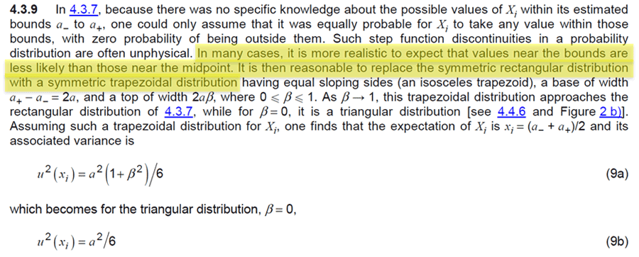
From the GUM statement, you can choose a triangle or trapezoid distribution instead of a rectangular distribution even though your uncertainty is estimated only by limits and you have no clue where the actual value is within the limits.

I prefer this alternative. I never liked using rectangular distributions where they are not likely to actually represent a population of data. However, there are plenty of others who disagree with me.

If you would like to use the trapezoid or triangle distribution instead of the rectangular distribution, here is what I recommend.

 
 

A) Triangle Distribution (Common)

Most uncertainty guides and papers make use of the triangle distribution, not the trapezoid distribution. So, I would recommend using the triangle distribution. However, most assessors want you to have evidence to support its use.

Therefore, I recommend reviewing your calibration certificates. If the calibration result is less than 50% of the tolerance limit, it is easy to claim that the value in the interval is closer to the midpoint than the limit. This should help you justify the use of the triangle distribution.

 
 

B) Trapezoid Distribution (Not Common)

If you want to use the trapezoid distribution (this is not common), I think there is a smart way to make use of it. Many labs will establish decision rules to adjust their equipment if the performance exceeds (for example) 70% of the tolerance limit (TL).

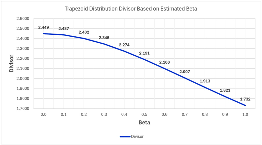
In this scenario, you use the tolerance limits as your uncertainty and characterize it with a trapezoid distribution where β=0.3 (i.e (100%-70%)/100=0.3). The divisor to convert your uncertainty contributor to a standard uncertainty is k=2.007.

This solution is similar to a normal distribution where you would expect most of your results to be within one standard deviation of the mean (i.e. 68% confidence level). For reference, a normal distribution with a 95% confidence level has a divisor of k=2.

However, due to the extra work to calculate the divisors and the lack of adoption in measurement uncertainty calculators and software, most people will not use this distribution.

In fact, I have never used it (yet) although I have considered it many times.

In case you want to use the trapezoid distribution, I have made a chart of the distribution’s divisors (to convert uncertainty to standard uncertainty or standard deviation equivalents) versus beta value.

In the chart below, you will notice that:

1. When beta is 0, the divisor is equal to a triangle distribution, and
2. When beta is 1, the divisor is equal to a rectangular distribution.

 
 

GUM Compromise: Triangle Distribution

Finally, I wanted to share an important recommendation in Appendix F of the JCGM 100:2008.

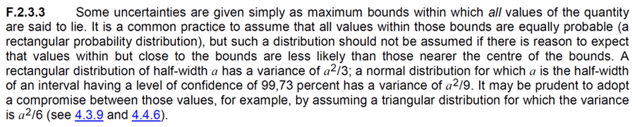
In section F.2.3.3, the GUM provides a compromise to disputes between assuming a normal and rectangular distribution. When there is a dispute, the guide recommends assuming a triangle distribution.

I wanted to share this recommendation, because I routinely have debates with assessors and other professionals about whether a tolerance or specification should be characterized by a normal or rectangular distribution.

If you find yourself in a debate, this section of the GUM may be helpful.

Look at the image below to see section F.2.3.3 in the JCGM 100:2008.

 
 

---

 
 

Probability Distributions Decision Tree and Tables

Before wrapping up this guide, I made a few decision tables and decision trees to help you pick appropriate probability distributions for your uncertainty budgets.

 
 

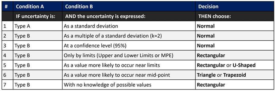
Decision Table Based on the GUM

The table below is a decision table based on recommendations in the GUM (JCGM 100:2008).

It makes a great cheat sheet to characterize sources of uncertainty by:

1. Uncertainty Type, and
2. Probability Distribution.

 

 
 

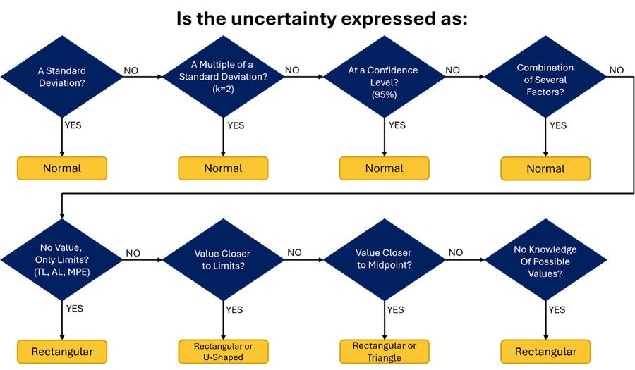
Decision Tree Based on the GUM

The decision tree or flow chart below is similar to the above decision table. It will help you pick a probability distribution based on recommendations in the GUM (JCGM 100:2008).

Simply start at the top-left of the decision and answer the questions moving left to right. Based on your answers, you will find the probability distribution for your uncertainty contributor.

If you prefer flow charts instead of tables, this will work better for you.

 
 

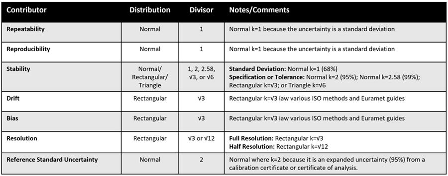
Decision Table for Common Sources of Uncertainty

Finally, you will find a decision table for common sources of uncertainty that I cover in many of my guides. These are the uncertainty contributors that I recommend you include in most uncertainty budgets. Therefore, I thought it would be helpful to have a decision table to help you pick the right probability distributions for each of these uncertainties.

To use the table, find the uncertainty contributor in the left-most column. Next, look at the distribution column (i.e. 2^nd column) on the same row to find the probability distribution that you should use.

If there is more than one option available, look at the Notes/Comments column (i.e. 4^th column) on the same row for information to help you choose the right distribution for your uncertainty.

Additionally, I included the divisors in the 3^rd column that you should use to convert your uncertainty contributor to a standard uncertainty. Again, if there is more than one option look at the Notes/Comment column on the same row to help you choose the right divisor.

This is great cheat sheet that I started including in my measurement uncertainty training last year.

 
 

---

 
 

Conclusion

Probability distributions are an important part of understanding the behavior of functions, analyzing sources of uncertainty, and predicting future outcomes. This is why they are a critical component of uncertainty analysis.

If you estimate measurement uncertainty without considering the probability distributions, you are going to make mistakes. Therefore, make sure to use this guide as a reference when making your uncertainty budgets.

In this guide, you should have learned the following:

1. What is a probability distribution,
2. Common distributions used in uncertainty analysis,
3. GUM recommendations for picking distributions, and
4. Decision trees and flow charts for selecting the right distribution.

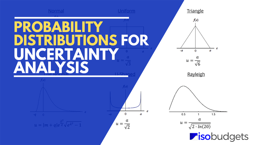
Finally, look at the image below. It is probability distribution cheat sheet with a summary of the distributions covered in this guide including the divisors and formulas needed to convert every one of your contributors to a standard uncertainty.

 
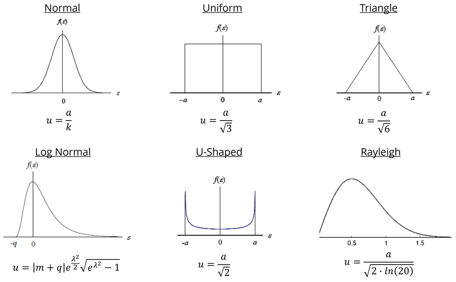
Overall, the information in this guide should help you confidently pick the right distributions next time your estimate uncertainty.

I hope that you have found this article helpful for your uncertainty analysis. Leave me a comment and tell me the probability distributions you use in your uncertainty analysis.

 
 

This article was originally published on October 28, 2015 and updated on March 8, 2024.

References

- JCGM. (2008). JCGM 100:2008(E) Evaluation of measurement data — Guide to the expression of uncertainty in measurement. Sèvres: JCGM.
- Castrup, H. (2007). Distributions for Uncertainty Analysis. Bakersfield, CA: Integrated Sciences Group.
- Castrup, H. (2009). Error Distribution Variances and Other Statistics. Bakersfield: Integrated Sciences Group.
- DeCarlo, L. T. (1997). On the Meaning and Use of Kurtosis. American Psychological Association Inc., 292-302.
- Keysight Technologies. (2014). Application Note 1449-3 Fundamentals of RF and Microwave Power Measurements (Part 3). Santa Rosa: Keysight Technologies.
- Dobbert, M., & Gorin, J. (2011). Revisiting Mismatch Uncertainty with the Rayleigh Distribution. Santa Rosa: Agilent.
- Petty, N. W., & Dye, S. (2013). Triangular Distributions. Christchurch: Statistics Learning Centre.
- NIST. (2012). NIST/SEMATECH e-Handbook of Statistical Methods, 1.3.6.6.9. Lognormal Distribution. Gaithersburg: NIST.