Key Takeaways: Combining Uncertainty
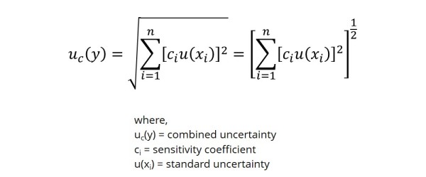
- Methodology: Components are combined using the Root Sum of the Squares (RSS) method, also known as the Law of Propagation of Uncertainty.
- Pre-requisite: All components must be expressed as standard uncertainties (u) in the same units before combining.
- Sensitivity Coefficients: Essential for converting different units (e.g., Temperature to Length) so they can be summed mathematically.
- Combined Standard Uncertainty (uc): Represents the estimated standard deviation of the result, typically at a 68% confidence level.
- ISO 17025 Requirement: Labs must use valid statistical methods (GUM) to combine all significant contributors identified in the budget.
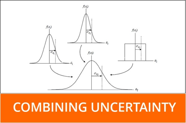
So, let’s assume that you are estimating measurement uncertainty. You have identified the influencing factors, quantified the magnitude of their contribution, and reduced them to a standard uncertainty. Now, if you are wondering what the next step is, it is to combine the independent uncertainty components to calculate ‘Combined Uncertainty.’ This is the step you will need to take before calculating ‘Expanded Uncertainty.’
The goal of combining uncertainty is to calculate the total magnitude of uncertainty from a set of independent uncertainty components, each with their own varying degrees of magnitude. It is a common process covered in the GUM and many other measurement uncertainty guides. However, I thought it would be a good idea to explain the process in a little more detail.
What is Combined Uncertainty
Combined Uncertainty is the square-root of the linear sum of squared standard uncertainty components. This method is also known as ‘Summation in Quadrature’ or ‘Root Sum of the Squares.’ Each component is the product (i.e. result of multiplication) of the standard uncertainty and its associated sensitivity coefficient. By combining these components, we are attempting to estimate the total magnitude of uncertainty associated with our evaluated measurement system or process.
“Standard uncertainties, both Type A and Type B, can be combined using a method known as ‘summation in quadrature’ or ‘root sum of the squares.” – Stephanie Bell
Why is Uncertainty Combined This Way
Summation in Quadrature
To best explain summation in quadrature, think Vector Addition and Pythagorean’s Theorem. If we treat uncertainty contributors as orthogonal (i.e. statistically independent), each as a vector with independent quantities of displacement/magnitude, then we can calculate the net displacement/magnitude by addition in quadrature.
Central Limit Theorem
When performing uncertainty analysis, we use a variety of probability densities/distributions to characterize each contributing factor. Some of the most common distributions used in uncertainty analysis are Gaussian (i.e. normal), uniform (i.e. rectangular), and triangular. When we combine these probability densities to calculate combined uncertainty, the resulting calculation is characterized by a normal distribution. Why? The Central Limit Theorem.
According to the Central Limit Theorem, the sum of a set of independent random variables will approach a normal distribution regardless of the individual variables distribution. This is why combined uncertainty is characterized by a normal distribution, even though we combined a several sets of data characterized by various distributions.
How to Combine Uncertainty
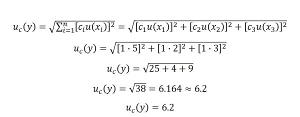
As explained earlier, uncertainty is combined using a method known as summation in quadrature. Below, I provided the formula and an example of combining uncertainty.
Example:
If we have three uncertainty components, each with a sensitivity coefficient of one (i.e. 1), the result would be:
c1 = 1
c2 = 1
c3 = 1
u(x1) = 5 ppm
u(x2) = 2 ppm
u(x3) = 3 ppm
If you are using Microsoft Excel to combine uncertainty, use the following formula to accomplish the task.
=sqrt(sumsq(Cell 1, Cell 2, …, Cell n))
The ‘sqrt‘ function calculates the square root of the data placed in between the parentheses. The next function, ‘sumsq‘ calculates the sum of squares. This function squares the value of each cell and then adds them all together, hence, the sum of squares. When these two functions are combined as I have shown, the result is the square root of the sum of squares or the root sum of the squares. Using this equation is much simpler and easier than squaring and adding each cell independently.
Hopefully, this post has been educational to some degree. Whether you are a beginner or an expert at uncertainty analysis, I hope that I have provided some beneficial information for you to take away from this post. If you have any questions or comments, please feel free to fill in the comments section below or email me at [email protected].
Want to learn more about combining uncertainty? Here are links to some good information. Enjoy!
http://www.isgmax.com/Articles_Papers/Estimating%20and%20Combining%20Uncertainties.pdf
https://www.wmo.int/pages/prog/gcos/documents/gruanmanuals/UK_NPL/mgpg11.pdf
http://ipl.physics.harvard.edu/wp-uploads/2013/03/PS3_Error_Propagation_sp13.pdf
https://physicscourses.colorado.edu/phys2150/phys2150_sp19/2150L3.pdf
http://mathworld.wolfram.com/Vector.html
http://web.mit.edu/fluids-modules/www/exper_techniques/2.Propagation_of_Uncertaint.pdf
http://mathworld.wolfram.com/CentralLimitTheorem.html
http://www.dartmouth.edu/~chance/teaching_aids/books_articles/probability_book/Chapter9.pdf


2 Comments