Key Takeaways: Effective Degrees of Freedom
- Definition: A measure used to determine the reliability of a combined uncertainty estimate, accounting for varying degrees of freedom in individual components.
- Welch-Satterthwaite Equation: The standard formula used to calculate $\nu_{eff}$ by combining the variances and individual degrees of freedom.
- Role in ISO 17025: Essential for determining the correct coverage factor ($k$) from the Student’s t-distribution when the effective degrees of freedom are less than infinite.
- Significance: A low νeff suggests that the uncertainty estimate is less reliable, requiring a larger expansion factor to achieve the 95% confidence level.
- Audit Expectation: Modern assessors look for this calculation when Type A components have a small sample size (e.g., n < 10).
Degrees of Freedom
Before getting ahead of ourselves, it is important to address degrees of freedom. In statistics, degrees of freedom is the number of values in the final calculation which are free to vary. In other words, it is the number of ways or dimensions an independent value can move without violating constraints.
To calculate degrees of freedom, subtract the number of relations from the number of observations. For determining the degrees of freedom for a sample mean or average, you need to subtract one (1) from the number of observations, n.
Take a look at the image below to see the degrees of freedom formula.
Effective Degrees of Freedom
Now that I have explained degrees of freedom, let’s look at effective degrees of freedom and the Welch Satterthwaite approximation equation.
When performing uncertainty analysis, you evaluate and combine multiple uncertainty components characterized by various probability distributions. Typically, this complex process causes the degrees of freedom to be inappropriate or undefined. Therefore, you need to calculate the effective or equivalent degrees of freedom, for inference purposes, to approximate the actual degrees of freedom.
This is accomplished using the Welch Satterthwaite equation. Essentially, it pools the degrees of freedom to give you an approximated average.
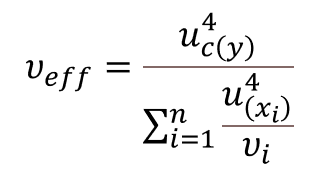
Take a look at the image below to see the effective degrees of freedom formula.
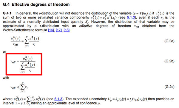
This is the same equation recommended by the JCGM 100:2008 – The Guide to the Expression of Uncertainty in Measurement (i.e. The GUM). Take a look at the image below for an excerpt from Appendix G of the GUM.
See How We Can Help Your Lab Get ISO/IEC 17025:2017 Accredited
- Uncertainty Budgets – let us estimate uncertainty for you.
- Custom QMS – we’ll create your quality manual, procedures, lists, and forms.
- Training – get online training that teaches you how to estimate uncertainty.
Applying the Equation
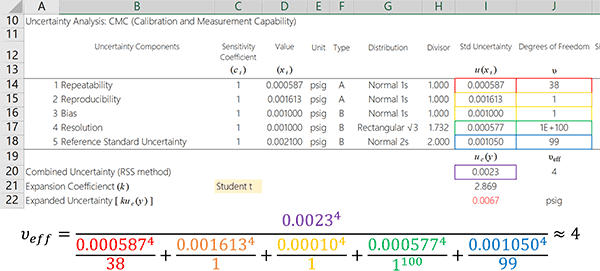
Using the equation given above and the table pictured below, you can see how to easily apply the equation to your uncertainty calculations. Take a look at the highlighted boxes. Each box is identified by color and symbol. Plug the values into the equation and calculate the effective degrees of freedom.
Otherwise, check out the next section to learn how to calculate the effective degrees of freedom step by step using Microsoft Excel.
How to Calculate the Effective Degrees of Freedom
Calculating the effective degrees of freedom with the Welch Satterthwaite equation can look confusing, so I am going to break the process down into easy to follow steps for you.
1. Raise each uncertainty component to the power of 41
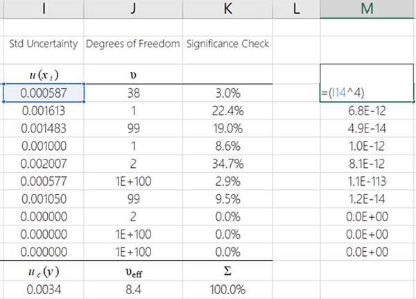
The first thing that want to do is raise each standard uncertainty component to the power of 4.
Take a look at the image below for the formula in MS Excel. After you finish raising the first uncertainty component to the power of 4, copy and paste the function for the remaining uncertainty components.
2. Divide each uncertainty by it’s associated degrees of freedom
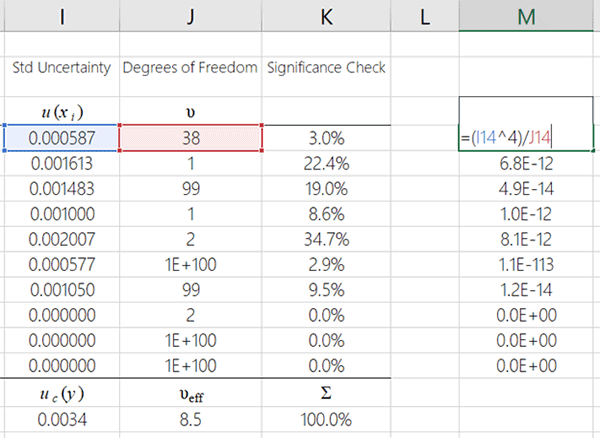
The second step you will take is to divide your previous result by it’s associated degrees of freedom.
Take a look at the image below to see how to perform this in MS Excel.
3. Add the results from the previous step,
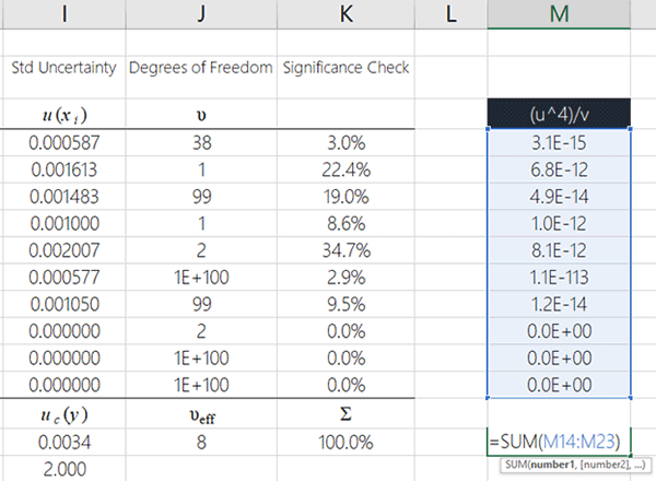
In this step, you want to add together all of your results from the previous step.
You can easily do this in MS Excel using the summation (i.e. SUM) function. Look at the image below to see how to do it.
4. Raise the combined uncertainty to the power of 4
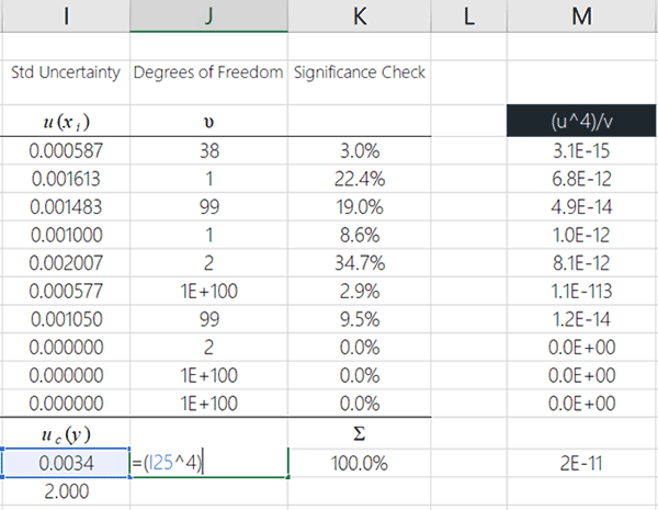
Now, you need to raise your combined standard uncertainty to the power of 4.
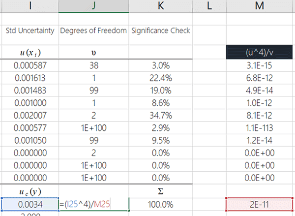
Take a look at the image below to see how to do this in Microsoft Excel. I recommend entering this function where you want to see the calculated effective degrees of freedom, because I am going to show you how to finish this process in the cell that you see in the image below.
5. Divide the result in step 4 by the result in step 3
Next, you will divide the result from the previous step by the result you calculated in step 3.
Take a look at the image below to see how to do in Microsoft Excel.
The result that you calculate is the effective degrees of freedom. However, you are not done yet. You will need to round the result to a whole number in the next step.
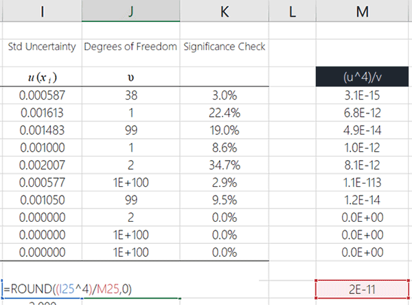
6. Round the result to the nearest whole number.
Finally, round the result to a whole number using the ROUND function in Microsoft Excel.
Look at the image below to see how to do it.
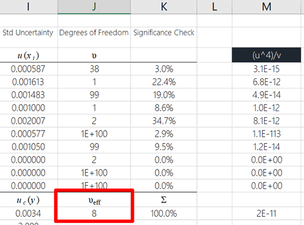
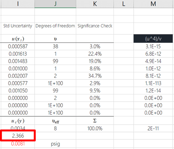
The Result
If you followed the steps above, you just calculated the effective degrees of freedom. Great job!
Take a look at the image below to see the final result.
Coverage Factor for Expanded Uncertainty
If you prefer to use the Student’s T table to find your coverage factor for calculating your expanded uncertainty, you can use the effective degrees of freedom (that you just calculated).
You will need to use the TINV function in Microsoft Excel.
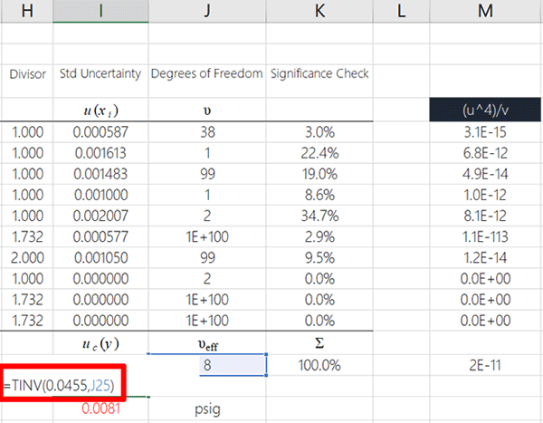
Take a look at the image below to see how to use the TINV function.
Find the Coverage Factor Using the TINV Function
All you need to do is:
- Select a cell to calculate your coverage factor,
- Type “=TINV(0.0455,” into the cell,
- Select the cell where your degrees of freedom is calculated,
- Type “)” and hit the Enter key.
Your result will be a 95% coverage factor based on the Student’s T table.
Finally, take a look a the image below to see the coverage factor that was found using the Student’s T table and the effective degrees of freedom.
Conclusion
Now that you know how to calculate the effective degrees of freedom and use the Welch Satterthwaite equation, feel free to try it out and include it in your uncertainty budgets. Many people struggle with this equation. So, I hope that you find this guide helpful. If you have any questions, please feel free to contact me.
If you want to learn more about the Welch Satterthwaite approximation equation, check the original papers published by F.E. Satterthwaite and the B.L. Welch.
The Generalization of `Student’s’ Problem when Several Different Population Variances are Involved
An Approximate Distribution of Estimates of Variance Components
Vol. 2, No. 6 (Dec., 1946), pp. 110-114
Published by: International Biometric Society
This article was originally published June 13, 2014, and updated June 11, 2021.




8 Comments