Methods for Determining the Coverage Factor k
According the the JCGM 100:2008 (GUM) Appendix G, there are two ways to determine the coverage factor k. These include:
- Method 1: Coverage Factor Table (JCGM 100:2008, section G.1.3):
- Method 2: T-distribution (JCGM 100:2008, section G.3):

Find the Coverage Factor using JCGM 100, Table G.1
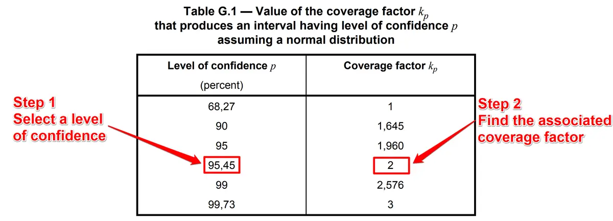
The fastest and easiest way to find the coverage factor k is to use Table G.1 in the JCGM 100:2008 (GUM). If your combined measurement uncertainty is a normal distribution, then this is the right method to use.
Follow the instructions below and refer to the image for clarification.
- Step 1: Select the desired level of confidence (e.g. 95.45 %).
- Use a 95.45 % level of confidence.
- Step 2: Find the associated coverage factor from JCGM 100:2008, Table G.1.
- Find the level of confidence in the left column.
- Find the associated coverage factor k in the right column.
To use this method, your combined measurement uncertainty must have a normal distribution and meet the conditions of the Central Limit Theorem. See JCGM 100:2008, section G.6.6.
Otherwise, you will need to determine the coverage factor k using the t-distribution.
Find the Coverage Factor using JCGM 100, Table G.2
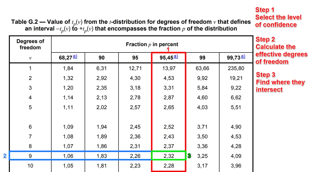
If your combined measurement uncertainty does not meet the conditions of the Central Limit Theorem (to assume a normal distribution), then determine the coverage factor k using the t-distribution.
Follow the instructions below and refer to the image for clarification.
- Step 1: Select the desired level of confidence. (e.g. 95.45 %).
- Use a 95.45 % level of confidence.
- Step 2: Calculate the effective degrees of freedom using the Welch-Satterthwaite formula (JCGM 100:2008, section G.4.1).
- Step 3: Use the Student’s t-distribution or table (JCGM 100:2008, table G.2) to obtain the coverage factor.
- Find the column that matches the level of confidence.
- Find the row that matches the degrees of freedom.
- Find the coverage factor k where they intersect.
FAQ
What is a coverage factor k?
A coverage factor is a multiplier that is used to expand measurement uncertainty to a desired level of confidence (e.g. 95 %).
What level of confidence should I estimate uncertainty to?
You should estimate uncertainty to a 95.45 % level of confidence.
According to the JCGM 100:2008, the GUM recommends estimating uncertainty at 95 to 99 % confidence intervals.
However, accredited laboratories (ISO/IEC 17025) and producers (ISO 17034) are expected to express uncertainty to an approximately 95 % confidence interval where k=2. When the coverage factor k=2, the level of confidence is 95.45 %.
Keep this in mind when determining the coverage factor k.
What is the Welch-Satterthwaite formula?
It is the formula used to estimate the effective degrees of freedom for the combined standard uncertainty, so the t-distribution can be used to find the coverage factor k to calculate the expanded uncertainty at a specific confidence level.
How to Calculate the Effective Degrees of Freedom?
Use the Welch-Satterthwaite formula given in the JCGM 100:2008, section G.4.1.
I have a guide that will show you how to calculate the effective degrees of freedom step-by-step. Click the link below to check it out.
How does confidence level relate to a coverage factor in ISO/IEC 17025?
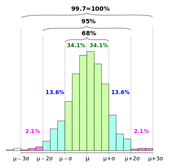
The confidence level is related to the Probability Distribution’s Density function and the number of standard deviations needed to obtain the desired percentage of the probability density function.
This is based on the Empirical Rule (i.e. 68-95-99 rule) in statistics. Look at the image below for an example:
Glossary
- Coverage Factor
- – number larger than one by which a combined standard measurement uncertainty is multiplied to obtain an expanded measurement uncertainty. (Source: JCGM 200:2012, 2.38)
- Level of Confidence
- the likelihood that a set of measurement values are contained within a specified coverage interval. (Source: JCGM 200:2012, 2.37)
- Effective Degrees of Freedom
- the degrees of freedom of the combined standard measurement uncertainty (uc) obtained from the Welch-Satterthwaite formula and used to determine the coverage factor (k) approximated by a t-distribution. (Source: JCGM 100:2008, G.4)
- Probability Distribution
- a function or table that describes the likelihood of all possible outcomes for a random variable associated with an experiment or event.
- Central Limit Theorem
- a concept in probability theory where the distribution of sample means will take the shape of a normal distribution regardless of the underlying distribution if the sample size is large enough.
- Empirical Rule
- a statistical principle that states for a normal distribution, approximately 68.27 % of outcomes will occur within one standard deviation, 95.45 % of outcomes will occur within two standard deviations, and 99.73 % of outcomes will occur within three standard deviations.
- Standard Measurement Uncertainty
- measurement uncertainty expressed as a standard deviation. (Source: JCGM 200:2012, 2.30)
- Expanded Measurement Uncertainty
- the product of a combined standard measurement uncertainty and a factor larger than the number one. (Source: JCGM 200:2012, 2.35)
- Combined Standard Measurement Uncertainty
- standard measurement uncertainty that is obtained using the individual standard measurement uncertainties associated with the input quantities in a measurement model. (Source: JCGM 200:2012, 2.31)