νi = 1/2 · [δu(xi)/u(xi)]-2
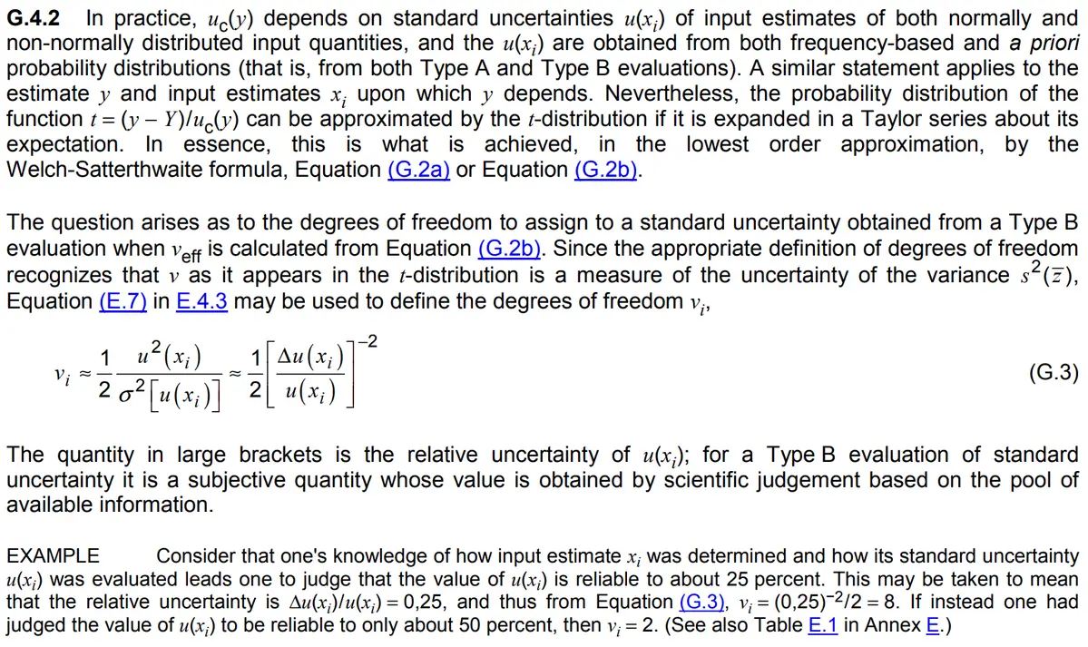
In the image below is an excerpt from the JCGM 100:2008 section G.4.2.
Type B Uncertainty with Infinite Degrees of Freedom
Typically, a Type B uncertainty evaluation is associated with infinite degrees of freedom.
According to the NIST SEMATECH Handbook, section 2.5.7.1 provides a list of example cases where Type B evaluations are assumed to have infinite degrees of freedom. These include:
- Worst-case estimate based on a robustness study or other evidence
- Estimate based on an assumed distribution of possible errors
- Type B uncertainty component for which degrees of freedom are not documented
GUM Method to Estimate Type B Uncertainty Degrees of Freedom
In the JCGM 100:2008 section G.4.2, the GUM recommends a formula to estimate the degrees of freedom for a Type B uncertainty based on a judgement of reliability similar to Table E.1 in Annex E.
The best way to implement this is to estimate your level of confidence in the value of the Type B uncertainty (e.g. 95 %). Then, calculate the reliability by subtracting 1 by the level of confidence (1 – 95/100 = 0.05).
Now, you can use the formula G.3 to estimate the degrees of freedom (υi = (0.05)-2/2 = 200).
Formula
Below, I have created a simplified version of the formula where p is the estimated level of confidence.

| Confidence | Reliability | Degrees of Freedom |
|---|---|---|
| 99 % | 0.01 | 5000 |
| 98 % | 0.02 | 1250 |
| 95 % | 0.05 | 200 |
| 90 % | 0.10 | 50 |
| 85 % | 0.15 | 22 |
| 80 % | 0.20 | 13 |
| 75 % | 0.25 | 8 |
| 70 % | 0.30 | 6 |
| 65 % | 0.35 | 4 |
| 60 % | 0.40 | 3 |
| 50 % | 0.50 | 2 |
| 40 % | 0.60 | 1 |
| 30 % | 0.70 | 1 |
| 20 % | 0.80 | 1 |
| 10 % | 0.90 | 1 |
FAQ
What is effective degrees of freedom?
Effective degrees of freedom (υeff) is an approximation of the degrees of freedom associated with the combined standard uncertainty. It is calculated using the Welch-Satterthwaite formula and used to quantify the reliability of the combined uncertainty estimate.
Why is the Welch-Satterthwaite formula used in uncertainty analysis?
The Welch-Satterthwaite formula is used to calculate the effective degrees of freedom so the coverage factor (k) can be determined using the Student’s t-distribution per JCGM 100:2008, Appendix G.
According to JCGM 100:2008 Appendix G.6.4, it is the preferred method to calculating the expanded uncertainty.
However, Appendix G.6.5 states this method is not recommended when the conditions of the Central Limit Theorem are not met. For example, when the combined standard uncertainty is dominated by an uncertainty contributor with a rectangular distribution.
Furthermore, Appendix G.6.6 provides a list of conditions that should be met to use effective degrees of freedom to determine the coverage factor (k).
More information can be found in JCGM 100:2008 sections G.3 and G.4.
How do you choose a coverage factor (k) for expanded uncertainty?
The coverage factor (k) is chosen based on the desired level of confidence (typically 95% or 95.45%) and one of the methods given in the JCGM 100:2008 Appendix G.
- Normal Distribution: Use JCGM 100:2008 Table G.1 to find the coverage factor (95.45% C.I., k=2) based on the z-factor of a normal distribution.
- Student’s t-Distribution: Use JCGM 100:2008 Table G.2 with the level of confidence and effective degrees of freedom to find the coverage factor (e.g. 95.45% C.I., υ=9, k=2.32) based on the t-factor of a Student’s t-distribution.
What is the relationship between the t-distribution and coverage factor?
The t-distribution is used to find the coverage factor (k) to calculate the expanded uncertainty. The coverage factor (k) is based on the critical t-factor determined by the t-distribution at a specified level of confidence and degrees of freedom.
Glossary
- Degrees of Freedom
- the degrees of freedom of the combined standard measurement uncertainty (uc) obtained from the Welch-Satterthwaite formula and used to determine the coverage factor (k) approximated by a t-distribution. (Source: JCGM 100:2008, G.4)
- Type B Uncertainty
- measurement uncertainty evaluated using techniques other than the statistical analysis of measurement or test results.
- Coverage Factor
- number larger than one by which a combined standard measurement uncertainty is multiplied to obtain an expanded measurement uncertainty. (Source: JCGM 200:2012, 2.38)
- Level of Confidence
- the likelihood that a set of measurement values are contained within a specified coverage interval. (Source: JCGM 200:2012, 2.37)
- Effective Degrees of Freedom
- an approximation of the degrees of freedom associated with the combined standard uncertainty. It is calculated using the Welch-Satterthwaite formula and used to quantify the reliability of the combined uncertainty estimate.
- Probability Distribution
- a function or table that describes the likelihood of all possible outcomes for a random variable associated with an experiment or event.
- Central Limit Theorem
- a concept in probability theory where the distribution of sample means will take the shape of a normal distribution regardless of the underlying distribution if the sample size is large enough.
- Empirical Rule
- a statistical principle that states for a normal distribution, approximately 68.27 % of outcomes will occur within one standard deviation, 95.45 % of outcomes will occur within two standard deviations, and 99.73 % of outcomes will occur within three standard deviations.
- Standard Measurement Uncertainty
- measurement uncertainty expressed as a standard deviation. (Source: JCGM 200:2012, 2.30)
- Expanded Measurement Uncertainty
- the product of a combined standard measurement uncertainty and a factor larger than the number one. (Source: JCGM 200:2012, 2.35)
- Combined Standard Measurement Uncertainty
- standard measurement uncertainty that is obtained using the individual standard measurement uncertainties associated with the input quantities in a measurement model. (Source: JCGM 200:2012, 2.31)