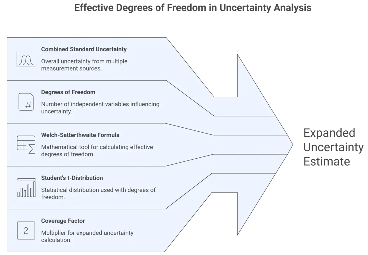
According the JCGM 100:2008, it is calculated with the Welch-Satterthwaite formula and used with the Student’s t-distribution to find a coverage factor (k) to calculate the expanded uncertainty at a specific confidence level (e.g. 95 % or 95.45 %) for ISO/IEC 17025 or ISO 17034 compliance.
Why Effective Degrees of Freedom is Important
Degrees of freedom are used as a metric for reliability and confidence in results. Typically, a larger effective degrees of freedom means the estimated measurement uncertainty is more reliable than a similar evaluation with less degrees of freedom.
For example, think about online reviews. If you are comparing two laboratories that both have a 5.0 ratings, who would you trust more – the lab with a 5.0 rating and only 10 reviews or a lab with a 5.0 rating and 1,000 reviews?
Usually, most people would answer the lab with 1000 reviews because 1000 review is a lot more than 10 reviews.
Effective degrees of freedom is similar. The more degrees of freedom, the more reliable the result.

Limitations of Effective Degrees of Freedom
Effective degrees of freedom has its limitations (as described in JCGM 100 sections G.2.3, G.5.4, and G.6.5). Since the calculation is heavily influenced by weighting the input uncertainties and it’s degrees of freedom, the effective degrees of freedom can be heavily skewed by one uncertainty contributor.
Dominant Uncertainty Contributors
According to JCGM 100 sections G.2.3 and G.6.5, the requirements of the Central Limit Theorem are not met when the combined standard uncertainty is dominated by:
- Type A uncertainty with just a few observations
- Type B uncertainty assumed to have a rectangular distribution.
If any of these scenarios occur, then it is recommended to use the coverage factor (k) from Table G.1.
For example, if a combined standard uncertainty is dominated by a Type B uncertainty with a rectangular distribution, then the effective degrees of freedom will closely agree with the dominating contributor. This can give a false representation of reliability (because the degrees of freedom are infinite) and result in an overstatement of the expanded uncertainty.
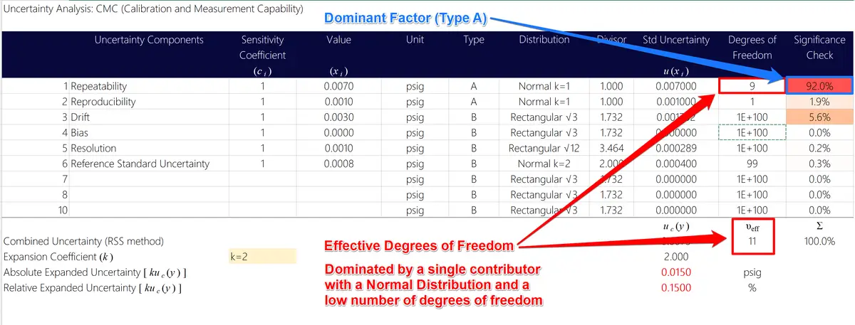
Dominant Type A Uncertainty
In the image below, you will see an example uncertainty budget where the effective degrees of freedom is dominated by a single Type A uncertainty with a small number of degrees of freedom. Notice the effective degrees of freedom closely matches the dominate Type A uncertainty.
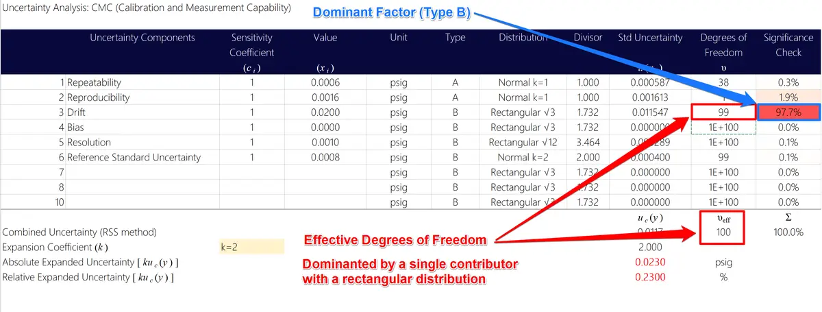
Dominant Type B Uncertainty
In the image below, you will see an example uncertainty budget where the effective degrees of freedom is dominated by a single Type B uncertainty with a rectangular distribution. Notice the effective degrees of freedom closely matches the dominate Type B uncertainty.
Other Limitations
Other limitations of the effective degrees of freedom and the t-distribution are provided in Appendix G of the JCGM 100, include:
- Non-normal distributions lead to incorrect coverage factors.
- The combined standard uncertainty must have a chi-distribution (Χ2) or the effective degrees of freedom is not valid.
- The result (y) must be independent of the combined standard uncertainty uc(y). Measurement functions with dependencies violate the requirements for using the t-distribution
- The degrees of freedom for Type B uncertainties are highly subjective which can lead small coverage factors and an underestimate of expanded uncertainty
Overall, the t-distribution is a preferred method to estimate the expanded uncertainty. However, take caution and use good judgement to avoid overestimating or underestimating expanded uncertainty.
FAQ
Why is the Welch-Satterthwaite formula used in uncertainty analysis?
The Welch-Satterthwaite formula is used to calculate the effective degrees of freedom so the coverage factor (k) can be determined using the Student’s t-distribution per JCGM 100:2008, Appendix G.
According to JCGM 100:2008 Appendix G.6.4, it is the preferred method to calculating the expanded uncertainty.
However, Appendix G.6.5 states this method is not recommended when the conditions of the Central Limit Theorem are not met. For example, when the combined standard uncertainty is dominated by an uncertainty contributor with a rectangular distribution.
Furthermore, Appendix G.6.6 provides a list of conditions that should be met to use effective degrees of freedom to determine the coverage factor (k).
More information can be found in JCGM 100:2008 sections G.3 and G.4.
How do you choose a coverage factor (k) for expanded uncertainty?
The coverage factor (k) is chosen based on the desired level of confidence (typically 95% or 95.45%) and one of the methods given in the JCGM 100:2008 Appendix G.
- Normal Distribution: Use JCGM 100:2008 Table G.1 to find the coverage factor (95.45% C.I., k=2) based on the z-factor of a normal distribution.
- Student’s t-Distribution: Use JCGM 100:2008 Table G.2 with the level of confidence and effective degrees of freedom to find the coverage factor (e.g. 95.45% C.I., υ=9, k=2.32) based on the t-factor of a Student’s t-distribution.
What is the relationship between the t-distribution and coverage factor?
The t-distribution is used to find the coverage factor (k) to calculate the expanded uncertainty. The coverage factor (k) is based on the critical t-factor determined by the t-distribution at a specified level of confidence and degrees of freedom.
Glossary
- Degrees of Freedom
- the degrees of freedom of the combined standard measurement uncertainty (uc) obtained from the Welch-Satterthwaite formula and used to determine the coverage factor (k) approximated by a t-distribution. (Source: JCGM 100:2008, G.4)
- Coverage Factor
- – number larger than one by which a combined standard measurement uncertainty is multiplied to obtain an expanded measurement uncertainty. (Source: JCGM 200:2012, 2.38)
- Level of Confidence
- the likelihood that a set of measurement values are contained within a specified coverage interval. (Source: JCGM 200:2012, 2.37)
- Effective Degrees of Freedom
- Probability Distribution
- a function or table that describes the likelihood of all possible outcomes for a random variable associated with an experiment or event.
- Central Limit Theorem
- a concept in probability theory where the distribution of sample means will take the shape of a normal distribution regardless of the underlying distribution if the sample size is large enough.
- Empirical Rule
- a statistical principle that states for a normal distribution, approximately 68.27 % of outcomes will occur within one standard deviation, 95.45 % of outcomes will occur within two standard deviations, and 99.73 % of outcomes will occur within three standard deviations.
- Standard Measurement Uncertainty
- measurement uncertainty expressed as a standard deviation. (Source: JCGM 200:2012, 2.30)
- Expanded Measurement Uncertainty
- the product of a combined standard measurement uncertainty and a factor larger than the number one. (Source: JCGM 200:2012, 2.35)
- Combined Standard Measurement Uncertainty
- standard measurement uncertainty that is obtained using the individual standard measurement uncertainties associated with the input quantities in a measurement model. (Source: JCGM 200:2012, 2.31)